goSPL-examples

Series of examples to illustrate the functionalities of goSPL.

goSPL (short for Global Scalable Paleo Landscape Evolution) is an open source, GPL-licensed library providing a scalable parallelised Python-based numerical model to simulate landscapes and basins reconstruction at global scale. goSPL is developed by the EarthCodeLab Group <https://earthcolab.org>_ at the University of Sydney.

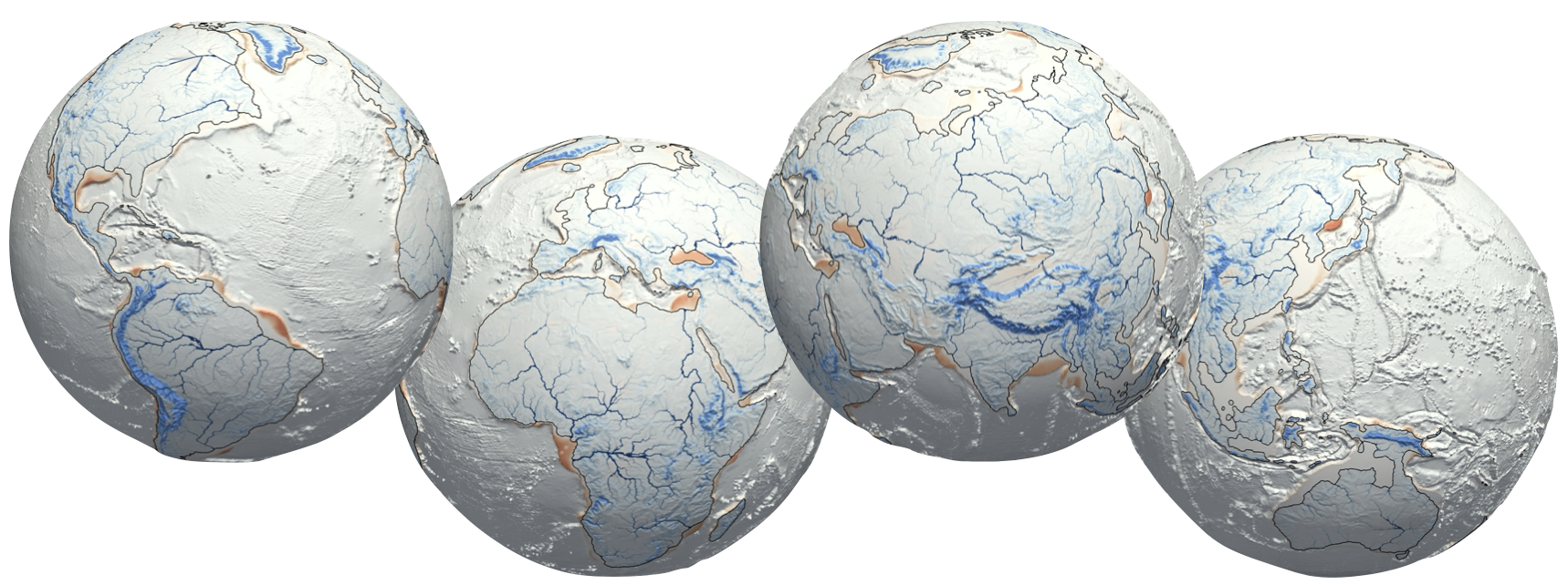
Full docs are available at: https://gospl.readthedocs.io/en/latest/

Installation via mamba / micromamba

We strongly recommend mamba or micromamba over plain conda: they use the fast libsolv resolver and reliably solve goSPL's heavy MPI/geospatial stack (the classic conda solver can stall or crash on it).

# with mamba
mamba env create -f environment.yml
mamba activate gospl-smoke

# or with micromamba (no base install needed)
micromamba create -f environment.yml
micromamba activate gospl-smoke

Plain conda env create -f environment.yml also works if you first enable the libmamba solver (conda install -n base conda-libmamba-solver && conda config --set solver libmamba); otherwise the classic solver may fail on this environment.

Here for more details.

Installation via Docker

The geodels/gospl-examples image packages the full gospl-smoke conda environment (goSPL, PETSc, GMT, VTK, JupyterLab) and is the recommended way to run the examples without a local conda install.

How the image is built. The image is built automatically from environment.yml (via mamba) by the Build and push Docker image GitHub Actions workflow and pushed to Docker Hub on every release tag or manual trigger. Two repository secrets are required: DOCKERHUB_USERNAME (a Docker Hub account with push access to geodels/gospl-examples) and DOCKERHUB_TOKEN (a Read & Write personal access token for that account, generated under Account Settings → Personal access tokens on Docker Hub).

Pulling the image

Once you have installed Docker on your system, pull the examples image:

docker pull geodels/gospl-examples:latest

Apple Silicon (M1/M2/M3) users. The image is published as a multi-arch manifest with native linux/arm64 and linux/amd64 builds, so a plain docker pull automatically selects the arm64 image on Apple Silicon — no --platform flag and no Rosetta emulation needed. Running the native arm64 image is much faster than forcing the amd64 image under emulation, so avoid adding --platform linux/amd64 on Apple Silicon. You can confirm you got the native build with:

docker run --rm geodels/gospl-examples:latest python -c "import platform; print(platform.machine())"
# expect: aarch64 on Apple Silicon, x86_64 on Intel

Starting the container from a terminal

Clone this repository and start the container, mounting it at /work:

git clone https://github.com/Geodels/goSPL-examples.git
cd goSPL-examples
docker run -it --rm -p 8888:8888 -v "$PWD":/work geodels/gospl-examples:latest

Apple Silicon users: no --platform flag is needed — Docker pulls the native linux/arm64 image automatically, which is significantly faster than amd64 emulation.

JupyterLab will start and print a http://127.0.0.1:8888/lab?token=… URL — open it in your browser. The full repository is visible under /work and the gospl-smoke environment is already active (no conda activate needed).

Depending on your operating system, you can configure Docker's resource allocation (CPUs, memory, swap, disk image size) to improve performance.

Note that you can also use the Docker Desktop Dashboard to pull the image instead of the terminal.

Running the examples with the gospl-examples image

The geodels/gospl-examples image ships the gospl-smoke environment only (no notebooks), so you run it against a local clone of this repository mounted at /work:

git clone https://github.com/Geodels/goSPL-examples.git
cd goSPL-examples
docker pull geodels/gospl-examples:latest
docker run -it --rm -p 8888:8888 -v "$PWD":/work geodels/gospl-examples:latest

JupyterLab starts and prints a http://127.0.0.1:8888/lab?token=… URL in the terminal — open it in your browser. Every example in the repository is visible under /work. Beyond the one shown below, the repo bundles a range of local and global examples, each pairing a pre-processing notebook (build_inputs.ipynb / model_setup.ipynb) with a post-processing notebook (view_Results.ipynb) — working through them is the best way to get familiar with goSPL's capabilities, so browse the examples catalog and pick any one.

Each example follows the same three stages:

1. Build the inputs — run all cells of the example's build_inputs.ipynb / model_setup.ipynb to generate the mesh and forcing files.
2. Run the model — open a terminal in JupyterLab (File ▸ New ▸ Terminal) and launch goSPL under MPI with the gospl command (below).
3. Analyse the outputs — run all cells of the example's view_Results.ipynb to remap and plot the results (these use the gospl-* post-processing tools — see Post-processing with the gospl-* tools).

# step 2, inside the container — here the stratigraphic_record example
cd /work/Local-examples/stratigraphic_record
mpirun -np 4 gospl -i input-strati.yml

gospl is the console entry point installed with the package (equivalent to the old python runModel.py). The gospl-smoke environment is already on the PATH (no conda activate needed) and the MPI/libfabric TCP workaround is baked into the image. Change -np 4 to the number of MPI ranks you want, and -i to the example's input file (add -v for verbose progress).

Performance — threading. The image defaults BLAS/OpenMP threads to 1 (OMP_NUM_THREADS, OPENBLAS_NUM_THREADS, MKL_NUM_THREADS, NUMEXPR_NUM_THREADS). goSPL gets its parallelism from MPI ranks (mpirun -np N), so single-threaded BLAS per rank avoids CPU oversubscription — leaving these unset lets every rank spawn one BLAS thread per core, which can make the container much slower than a native run. Set -np to the number of physical cores you want to use. For a non-MPI, single-process numpy/numba workload you can re-enable threading with e.g. docker run -e OMP_NUM_THREADS=8 .... Also make sure Docker Desktop is allocated enough CPUs/RAM (Settings → Resources).

Quick end-to-end test (no notebook required)

The stratigraphic_record example ships its inputs (inputs/gospl_mesh.npz, inputs/sealevel.csv), so you can run goSPL headless to verify the whole stack in a single command:

docker run -it --rm -v "$PWD":/work geodels/gospl-examples:latest \
  bash -lc "cd /work/Local-examples/stratigraphic_record && mpirun -np 4 gospl -i input-strati.yml"

A successful run prints goSPL's per-step progress and writes its HDF5 outputs into the example folder, ready to be post-processed by view_Results.ipynb. (The continental_flux example needs its build_inputs.ipynb run first, because its mesh is generated from the data/*.nc files.)

Detailed Conda installation

One of the simplest way to install not only goSPL, but required dependencies is with Anaconda, a cross-platform (Linux, Mac OS X, Windows) Python distribution for data analytics and scientific computing.

For Windows users, you will need to install Anaconda via the Windows Ubuntu Terminal from WSL. There are several articles on the web to do so (such as this one)

A full list of the packages available as part of the Anaconda distribution can be found here.

Another advantage to installing Anaconda is that you don't need admin rights to install it. Anaconda can install in the user's home directory, which makes it trivial to delete Anaconda if you decide (just delete that folder).

After getting Anaconda installed, the user will have already access to some essential Python packages and will be able to install a functioning goSPL environment by following the directives below.

Building goSPL-examples environment

The next step consists in downloading the conda environment for goSPL. A conda environment is like a virtualenv that allows you to install a specific flavor of Python and set of libraries. For the latest version (master branch) of goSPL, this is done by downloading the environment.yml file <https://raw.githubusercontent.com/Geodels/goSPL-examples/master/environment.yml>_. To do this you can use the curl:

  curl https://raw.githubusercontent.com/Geodels/goSPL-examples/master/environment.yml --output environment.yml

or wget command:

  wget https://raw.githubusercontent.com/Geodels/goSPL-examples/master/environment.yml

This will save the file locally under the same name as it was on github: environment.yml.

Alternatively you can get it from your preferred web browser by clicking on the following link: environment.yml and saving it under the following name environment.yml.

goSPL is not directly packaged as a Conda library because some of its dependencies are not available via this installation. The use of the environment file however provides an easy installation approach.

Once the environment.yml file has been downloaded on your system. The following directives provide a step-by-step guide to create a local conda environment for goSPL.

Navigate to the directory containing the environment.yml file and create the environment with mamba (or micromamba) — these are much faster and more reliable than plain conda on goSPL's MPI/geospatial stack:

    mamba env create -f environment.yml       # or:  micromamba create -f environment.yml

This will create an environment with the dependencies and packages required to run goSPL-examples.

To put your self inside this environment run::

    mamba activate gospl-smoke                 # or:  micromamba activate gospl-smoke

To install other packages, jupyter for example::

    mamba install jupyter

If you only have conda, first enable the fast solver — conda install -n base conda-libmamba-solver && conda config --set solver libmamba — otherwise the classic solver can fail to resolve this environment.

After your environment has been activated, you can either use VS-code or jupyter for running those examples on your local computer.

Repository structure

Each example lives in its own folder and follows the same three-stage workflow:

1. build_inputs.ipynb / model_setup.ipynb — build the mesh and the forcing fields (elevation, rainfall, tectonics, sea level) and export them as the .npz / netCDF files goSPL reads.
2. gospl -i input-*.yml — run the model from its YAML configuration with the gospl console command, optionally under MPI (mpirun -np N gospl -i input-*.yml).
3. view_Results.ipynb — post-process the HDF5 outputs with the gospl-* tools (remap to a regular grid / NetCDF, extract elevation, erosion–deposition erodep, flow accumulation, per-basin flux, stratigraphy) and visualise the results.

Mesh-building helpers shared across examples live in shared_scripts/umeshFcts.py (ufcts); the post-processing that used to sit in shared_scripts is now provided by goSPL's installed gospl-* console tools (see below).

Global examples

Example	What it demonstrates
continental_flux	Global continental erosion–deposition and sediment flux to the oceans over 1 Myr on a coastline-refined mesh.
erodep_1My	Global 1 Myr run coupling stream-power erosion, marine deposition and flexural isostasy.
plate_mvt	Global landscape evolution driven by horizontal plate motion (advection) together with vertical tectonics.
continental_geochem	Global climate-zoned solute geochemistry: latitudinal provinces each shed a characteristic species (tropical iron/ferricrete, subtropical-arid carbonate/calcrete, temperate silica/silcrete) under temperature-driven (Arrhenius) weathering, with a capillary-fringe duricrust and per-basin / per-species dissolved-load delivery to the ocean.

Local examples

Example	What it demonstrates
generate_2Dmesh	Building 2D unstructured (Voronoi / UGRID) meshes and goSPL input files, including from a GeoTIFF DEM.
flow_direction	Comparison of flow-routing schemes — single-flow (SFD), two-neighbour and multiple-flow-direction (MFD).
implicit_timestepping	Sensitivity of the implicit solver to the time step Δt (500 yr → 5 kyr): stability versus accuracy.
escarpment_retreat	Retreat of a rifted-margin escarpment under fluvial incision, hillslope diffusion, orographic rain and flexure.
glacial_erosion	Glacial erosion coupled with river/soil transport and critical-slope diffusion.
soil_generation	Soil production from bedrock weathering coupled with river transport and hillslope diffusion.
stratigraphic_record	Building a passive-margin model that records stratigraphy, then extracting stratal architecture and a Wheeler (chronostratigraphic) chart.
dual_lithology	Dual-lithology (coarse/fine) erosion–deposition with sediment-provenance tracking — attributes deposited sediment back to its source region.
groundwater_geochem	Water table + capillary-fringe duricrust (erodibility armoring) + Level-B conservative solute geochemistry (two tracers: dissolution → transport → precipitation → river/ocean export).
ferricrete_inversion	Two-stage tropical laterite relief inversion: a broad iron ferricrete cuirasse blankets a wet plain (water table + capillary-fringe duricrust, relative accumulation), then base-level fall dissects it and the armoured divides are left standing as ferricrete-capped mesas (relief grows ~30 → ~640 m).
valley_ferricrete	Absolute-accumulation valley ferricrete: the discharge_gate confines the crust to groundwater discharge zones (valley floors, footslopes) so it tracks the drainage network instead of blanketing the plain, while the un-precipitated dissolved iron is exported down the rivers — the lateral-accumulation counterpart to ferricrete_inversion.

Running via GitHub Codespaces

For a zero-install option, this repo has a .devcontainer/devcontainer.json that builds the same gospl-smoke environment straight from the Dockerfile and launches JupyterLab automatically — no local Docker or conda needed.

Billing. Codespaces usage here is billed to the account that creates the codespace (not the Geodels org), using that account's own included quota/plan — this repo doesn't have organization-level prebuilds or spending configured.

Starting a Codespace

Click the badge above, or from the repo's green Code button choose the Codespaces tab → Create codespace on main. GitHub builds the container (a few minutes on first launch — the mamba env create step is the same one described under Installation via Docker) and opens a browser-based VS Code with the repo mounted at /work.

First-launch time. Codespaces builds the container directly from the Dockerfile on every fresh launch — there's no prebuild caching on this repo, so expect the full mamba env create solve (several minutes, same as the first docker pull/build described under Installation via Docker) before JupyterLab is reachable. Once created, a given Codespace can be stopped and restarted without re-running the build (see the stopping/costs note further below), so this wait is only on first creation, not every time you resume.

Once the container is running, JupyterLab is already active on port 8888 in the background, but it won't auto-open — you land directly in the Codespaces/VS Code interface. To use JupyterLab, open the Ports tab (bottom panel), find port 8888, and click the globe icon to open it in a browser; the http://.../lab?token=… URL (with token) is available there or in the container log if you'd rather copy it directly (View ▸ Output).

The gospl-smoke environment is already active — same as the Docker image, no conda activate needed — and every example is visible under /work. Follow the same three-stage workflow described in Running goSPL-examples: build inputs, run gospl under MPI from a terminal, then post-process in view_Results.ipynb.

Compute. hostRequirements in the devcontainer requests a 4-core / 8GB machine. Free/personal GitHub accounts may be capped at smaller machine types regardless — check your Codespaces billing plan if launches get capped to 2 cores, since some of the global examples are memory-hungry.

Stopping / costs. Codespaces bill by compute-hour while running. Stop the Codespace from the codespace list (or it auto-suspends after a period of inactivity) to avoid unnecessary usage.

Running goSPL-examples

The examples provided here target the 2026.7.14 goSPL release (see environment.yml) and consist of simple local and global models that illustrate the main capabilities of the code. If you are new to goSPL, start with the local example stratigraphic_record and the global example continental_flux.

A typical run, from an activated environment, builds the inputs in the relevant notebook, then launches the model from a terminal with the gospl command, and finally post-processes the outputs in view_Results.ipynb:

mamba activate gospl-smoke          # or: micromamba activate gospl-smoke
cd Local-examples/stratigraphic_record
mpirun -np 4 gospl -i input-strati.yml

gospl is the console entry point installed with the package. Replace 4 with the number of MPI processes to use and input-strati.yml with the example's input file. Add -v for verbose output; gospl --help lists all options (--log, --profile, --version).

Post-processing with the gospl-* tools

Installing goSPL also installs a set of console commands for post-processing the HDF5 outputs — these are what the view_Results.ipynb notebooks call under the hood, and they can also be run standalone from a terminal. Append --help to any of them for the full option list.

Command	Purpose & example
gospl-grid	Remap goSPL outputs onto a regular grid / NetCDF (elevation, erodep, flow accumulation, chi, …). gospl-grid --h5dir out/h5 --mesh mesh.npz --out surface.nc
gospl-section	Stratigraphic cross-sections and Wheeler (chronostratigraphic) diagrams. gospl-section --h5dir out/h5 --mesh mesh.npz --kind cross --out section.pdf
gospl-strata-volume	Export the stratigraphic mesh / per-layer volumes. gospl-strata-volume --h5dir out/h5 --outdir strata
gospl-catchment	Per-basin water and sediment outflow from a gridded NetCDF. gospl-catchment -i surface.nc -o catchments.nc
gospl-provenance	Sediment-provenance attribution (source region → sink). gospl-provenance --mesh-npz mesh.npz --h5dir out/h5 --steps 0:50 --source source.npz
gospl-ela	Equilibrium-line-altitude (ELA) field from a temperature map. gospl-ela --temperature temp.npz